Pythonで離散時間フーリエ変換を実装

Pythonで離散時間フーリエ変換(DTFT, Discrete-Time Fourier Transform)と離散時間フーリエ逆変換を実装してみます。

アルゴリズム

離散時間フーリエ変換 (DTFT)

離散時間データを周波数データへ変換するDTFTの式は(1)で計算できます。

$$X[\omega] = \sum_{n=-\infty}^\infty x[n] \exp(-j \omega n) \tag{1}$$

(1)式の左辺の\(\omega\)を指定することで、その\(\omega\)におけるDTFTの値を計算することが出来ます。DTFTの結果は連続時間になるので、\(\omega\)は実数で指定できます。

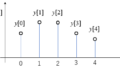
離散時間データは次のようなものです。(1)式は\(-\infty\)から\(\infty\)まで総和を計算していますが、離散データは有限なので、例えば以下の図のようなデータであれば、総和は”0″から”4″までを利用します。

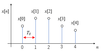
横軸はデータをサンプリング時間\(T_0\)で取得した値です。つまり \(n=0,1,2,3,4\)は時間ではなくデータのカウント数です。これを正規化時間と呼びます。実際のデータの時間は\(nT_0[sec]\)です。

それから、変換を行った\(X[\omega]\)の横軸も正規化時間をもとに計算しているので、正規化角周波数\(\omega\)[rad/sample]になります。正規化角周波数\(\omega\)は1サンプリング時間\(T_0\)毎に何\(rad\)進むかを表す値です。正規化されていない角周波数\(\Omega[rad]\)への変換は

$$
\Omega = \omega / T_0
$$

で計算します。

そして、DTFTは\([-\pi, \pi]\)で周期的な結果となります。

離散時間フーリエ逆変換 (IDTFT)

周波数データを離散時間データへ変換するIDTFTは(2)式で計算できます。

$$
x[n] = \frac{1}{2\pi} \int_{-\pi}^{\pi} X[\omega] \exp(j \omega n) d\omega \tag{2}
$$

(2)式の左辺の\(n\)を指定して、右辺の積分計算を行います。

積分計算はコンピュータで計算するには厄介ですが、数値積分のシンプソンの公式を使って行います。

アルゴリズム実装

使用するモジュール

複素数の計算が含まれているため、”cmath”モジュールを使用します。

import numpy as np
import cmath
import matplotlib.pyplot as plt # 結果表示用

離散時間フーリエ変換 (DTFT)

$$X[\omega] = \sum_{n=-\infty}^\infty x[n] \exp(-j \omega n)$$

# 離散時間フーリエ変換関数
def DTFT(omega, xn):
    _Xw = np.zeros(len(omega), dtype = np.complex)
    
    for i, w in enumerate(omega):
        for n, xn_i in enumerate(xn):
            _Xw[i] += xn_i * cmath.exp(-1j * w * n)
    
    return _Xw

この関数の戻り値は複素数型です。

離散時間フーリエ逆変換(IDTFT)

$$
x[n] = \frac{1}{2\pi} \int_{-\pi}^{\pi} X[\omega] \exp(j \omega n) d\omega
$$

# nを指定して、シンプソンの公式で逆離散時間フーリエ変換を計算
def InvertWithSimpsonRule(Xomega,omega_array,n):
    lim_n = int(len(Xomega)/2)
    h = abs(omega_array[1] - omega_array[0])
    
    sum = np.zeros(1, dtype=complex)
    for i in range(1, lim_n):
        f1 = (Xomega[2*i - 2] * (cmath.exp((1j) * omega_array[2*i - 2] * n )) )
        f2 = (Xomega[2*i - 1] * (cmath.exp((1j) * omega_array[2*i - 1] * n )) )
        f3 = (Xomega[2*i - 0] * (cmath.exp((1j) * omega_array[2*i - 0] * n )) )
        sum[0] += h*(f1 + 4*f2 + f3)/3

    
    return sum[0] / (2 * cmath.pi)

# nを変化させながら離散時間フーリエ逆変換計算
def InverseDTFT(omega_array, Xw_array, n_array):
    xn = np.zeros(len(n_array), dtype=np.complex)
    for n, n_atom in enumerate(n_array):
        xn[n] = InvertWithSimpsonRule(Xw_array, omega_array, n)
        
    return xn

この関数の戻り値は複素数型です。

周波数データ表示関数

離散時間フーリエ変換のデータを表示する関数も作成しておきます。この関数の引数’normalize’と’samplingTime’で、表示する離散時間フーリエ変換の横軸データを正規化角周波数[rad]から周波数[Hz]へ変換します。

import math
from matplotlib.ticker import (MultipleLocator, AutoLocator)

# 離散時間フーリエ変換データ表示関数
def showDTFTData(omega, Xw, normalize=True, SamplingTime = 1):
    fig = plt.figure(figsize=(12,5))
    ax = fig.add_subplot(111)
    if normalize:
        plt.plot(omega,Xw)
        plt.xlabel('Normalized angular frequency[rad]')
        plt.ylabel('X($\omega$)')
        ax.xaxis.set_major_locator(MultipleLocator(np.pi))
    else:
        x_data_hz = omega/SamplingTime/(2*np.pi) 
        plt.plot(x_data_hz ,Xw)
        plt.xlabel('Frequency[Hz]')
        plt.ylabel('abs(X($\omega$))')
        
        xtick = x_data_hz[-1]/10
        
        if xtick >= 1:
            ax.xaxis.set_major_locator(MultipleLocator(xtick))
        else:
            ax.xaxis.set_major_locator(AutoLocator())
        plt.minorticks_on()
        plt.grid(b=True, which='minor', color='#999999', linestyle='-', alpha=0.2)
        
    plt.grid(which='major', color='#666666', linestyle='-')
    plt.show()

離散時間データ表示関数

合わせて離散時間データ表示関数も定義します。

# 離散データ表示用関数
def showDiscreteData(x,y):
    markerline, stemline, baseline = plt.stem(x, y)
    plt.setp(markerline, marker='o', markeredgewidth=2, markersize=8, color='black', markerfacecolor='white', zorder=3)
    plt.setp(stemline, color='black', zorder=2, linewidth=1.0)
    plt.setp(baseline, color='black', zorder=1)
    plt.grid(True)
    plt.xlabel('n')
    plt.ylabel('y [n]')
    plt.show()

実装を行った関数で計算

用いる離散時間データ

# 離散時間データの定義
xd = np.array([0,0,1,1,1,0,0,0])
n = np.arrange(start = 0, stop = len(xd))

# 離散時間データの表示
showDiscreteData(n, xd)

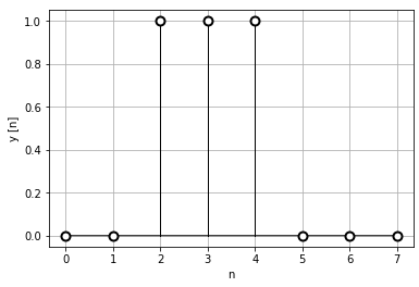
データを直接’np.array’で作成しているので、正規化時間データになっているように考えます。

離散時間フーリエ変換計算

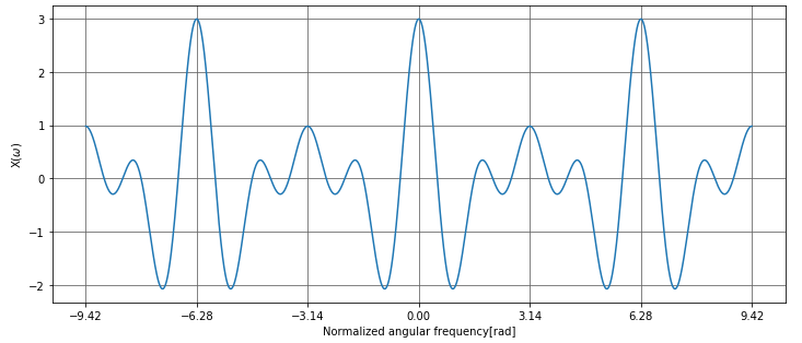
# DEFTの計算に用いる周波数 omega の範囲を指定
omega = np.linspace(-3*3.14, 3*3.14, 2020)

# 離散時間フーリエ変換の計算
Xw = DTFT(omega, xd)

# フーリエ変換結果の表示
showDTFTData(omega, Xw.real)

\(\pi\)毎にグリッドを表示しています。これで、\([-\pi, \pi]\)毎に周期的な結果となっていることが分かります。横軸は正規化角周波数となっていることに注意してください。

そして、DTFTの結果は複素数なので、showDTFTData関数の引数へは、’.real’で実部のみを抽出したデータを渡しています。今回は実部を表示していますが、この表示方法は複素数なので、実部、虚部、絶対値の３種類が考えられます。

離散時間フーリエ逆変換の計算

離散時間フーリエ逆変換は区間\([-\pi, \pi]\)の積分計算なので、もう一度範囲を\([-\pi, \pi]\)で離散時間フーリエ変換を行ったデータを用います。

# DEFTの計算に用いる周波数 omega の範囲を指定
omega = np.linspace(-1*3.14, 1*3.14, 2020)

# 離散時間フーリエ変換の計算
Xw = DTFT(omega, xd)

# 離散時間フーリエ逆変換の計算
i_xd = InverseDTFT(omega, Xw, n)

# 逆フーリエ変換結果の表示
showDiscreteData(n, i_xd.real)

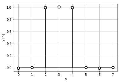
InverseDTFT関数の戻り値は複素数型なので、showDiscreteData関数の引数には’.real’で実数部を与えています。これは、もともとのデータに虚数が含まれていないからですね。

試しにshowDiscreteData()の第二引数に”i_xd.imag”で虚数部を与えてグラフを表示すると、以下の図のようにほぼゼロです。

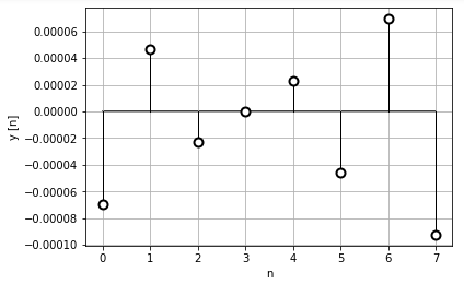
離散時間逆フーリエ変換の結果は、元のデータと比べて若干ずれは生じていますが、信号を再生できていると考えられる結果だと思います。

離散時間フーリエ逆変換の実装でシンプソンの公式を用いたので、数値計算誤差が生じた結果です。

でもしかし、離散時間フーリエ変換と離散時間フーリエ逆変換のアルゴリズムの確認をこれで出来ました。今回でアルゴリズムの確認が出来たので、次回はいろいろな信号に離散時間フーリエ変換を試してみます。