色々な離散データの離散時間フーリエ変換を計算してみる

離散時間フーリエ変換の実装が出来たので、色々な離散データを変換してみます。

離散時間フーリエ変換のクラス実装

離散データを入力して自動的に離散時間フーリエ変換を計算するクラスを作成します。

流れは、

(1) クラスを離散データでインスタンス化
(2) “.auto()”関数で以下の流れを実行
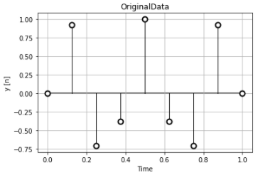
(2-1) 入力した離散データを表示
(2-2) 正規化された離散データを表示
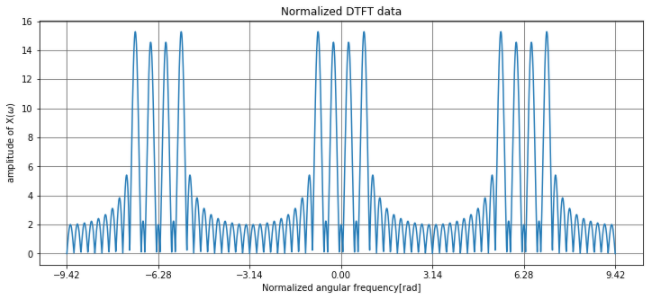
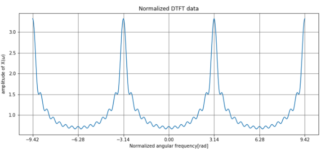
(2-3) 3周期分の離散時間フーリエ変換を計算し正規化角周波数[rad]で表示
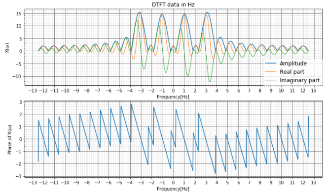
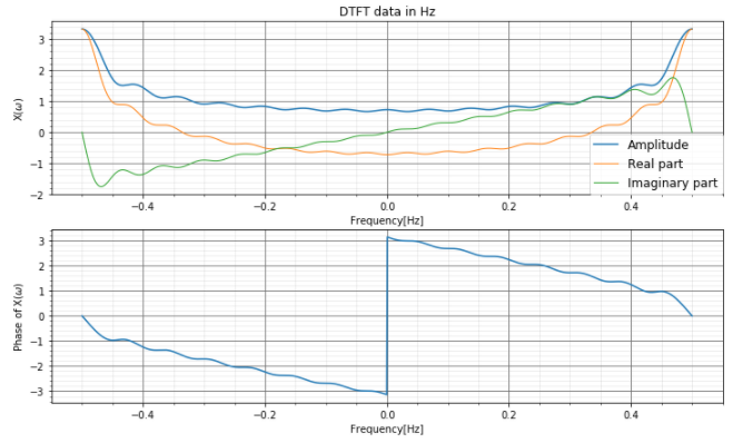
(2-4) 1周期分の離散時間フーリエ変換を計算し非正規化周波数[Hz]で表示
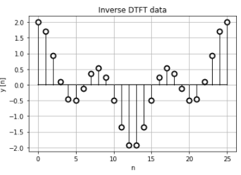
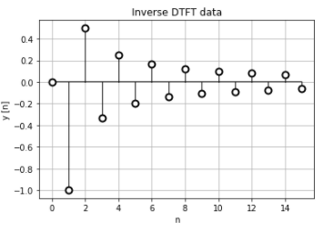
(2-5) 1周期分の離散時間フーリエ変換のデータから離散時間フーリエ逆変換を計算して表示

離散時間フーリエ変換をして、その計算結果が元の離散データに戻るかを離散時間フーリエ逆変換を行って確認してみる、という流れです。

import numpy as np
import cmath
import math
import matplotlib.pyplot as plt
from matplotlib.ticker import (MultipleLocator, AutoLocator)

class DTFTManager:
    # コンストラクタ
    def __init__(self, time_array = [0,1], xn_array = [0,1], xtick=1):
        self.time = time_array
        self.n_array = np.arange(len(time_array))
        self.xn = xn_array
        self.samplingTime = np.abs(time_array[0] - time_array[1])
        self.xtick = xtick
        
        self.omega_range_3 = np.linspace(-3*np.pi, 3*np.pi, 2020)
        self.omega_range_1 = np.linspace(-1*np.pi, 1*np.pi, 1000)
        
    # 離散時間フーリエ変換
    def DTFT(self, omega_array, xn_array):
        Xw = np.zeros(len(omega_array), dtype = np.complex)
    
        for i, w in enumerate(omega_array):
            for n, xn_atom in enumerate(xn_array):
                Xw[i] += xn_atom * cmath.exp(-1j * w * n)
    
        return Xw
    
    # シンプソンの公式で区間[-pi, pi]の積分を行う
    def __InvertWithSimpsonRule(self, omega_array, Xw_array ,n):
        lim_n = int(len(Xw_array)/2)
        h = abs(omega_array[1] - omega_array[0])
    
        sum = np.zeros(1, dtype=complex)
        for i in range(1, lim_n):
            f1 = (Xw_array[2*i - 2] * (cmath.exp((1j) * omega_array[2*i - 2] * n )) )
            f2 = (Xw_array[2*i - 1] * (cmath.exp((1j) * omega_array[2*i - 1] * n )) )
            f3 = (Xw_array[2*i - 0] * (cmath.exp((1j) * omega_array[2*i - 0] * n )) )
            sum[0] += h*(f1 + 4*f2 + f3)/3

        return sum[0] / (2 * cmath.pi)
    
    # 離散時間フーリエ逆変換
    def InverseDTFT(self, n_array, omega_array, Xw_array):
        
        xn = np.zeros(len(n_array), dtype=np.complex)
        for n, n_atom in enumerate(n_array):
            xn[n] = self.__InvertWithSimpsonRule(omega_array, Xw_array, n)

        return xn
    
    # 離散データ表示用関数
    def showDiscreteData(self, x,y,  graphTitle, normalize = True, SamplingTime = 1):
        
        if normalize:
            x_data = np.arange(len(x))
            x_label = 'n'
        else:
            x_data = x
            x_label ='Time'

        markerline, stemline, baseline = plt.stem(x_data, y)
        plt.setp(markerline, marker='o', markeredgewidth=2, markersize=8, color='black', markerfacecolor='white', zorder=3)
        plt.setp(stemline, color='black', zorder=2, linewidth=1.0)
        plt.setp(baseline, color='black', zorder=1)
        plt.title(graphTitle)
        plt.grid(True)
        plt.xlabel(x_label)
        plt.ylabel('y [n]')

        
        plt.show()
        
    # 離散時間フーリエ変換データ表示関数
    def showDTFTData(self, omega, Xw, graphTitle, normalize=True, SamplingTime = 1):
        absXw = np.zeros(len(Xw))
        phaseXw = np.zeros(len(Xw))
        myabs = np.zeros(len(Xw))
        for i, xw_ele in enumerate(Xw):
            absXw[i] = abs(xw_ele)
            phaseXw[i] = cmath.polar(xw_ele)[1]
            
        if normalize:
            fig = plt.figure(figsize=(12,5))
            ax1 = fig.add_subplot(111)

            ax1.plot(omega,absXw)
            ax1.set_xlabel('Normalized angular frequency[rad]')
            ax1.set_ylabel('amplitude of X($\omega$)')
            ax1.xaxis.set_major_locator(MultipleLocator(np.pi))
            ax1.grid(which='major', color='#666666', linestyle='-')
            ax1.set_title(graphTitle)

        else:
            fig = plt.figure(figsize=(12,7))
            # DTFTデータの振幅グラフ表示
            ax1 = fig.add_subplot(211)
            x_axis_data = omega/(SamplingTime*(2*np.pi)) # 非正規角周波数から周波数[Hz]を計算
            ax1.plot(x_axis_data ,absXw, label="Amplitude")
            ax1.plot(x_axis_data ,Xw.real, lw=1, label="Real part")
            ax1.plot(x_axis_data ,Xw.imag, lw=1, label="Imaginary part")

            ax1.set_xlabel('Frequency[Hz]')
            ax1.set_ylabel('X($\omega$)')
            ax1.set_title(graphTitle)
            ax1.legend(bbox_to_anchor=(1, 0), loc='lower right', borderaxespad=0, fontsize=12)
            if x_axis_data[-1] < self.xtick:
                ax1.xaxis.set_major_locator(AutoLocator())
            else:
                ax1.xaxis.set_major_locator(MultipleLocator(self.xtick))
            plt.minorticks_on()
            ax1.grid(b=True, which='minor', color='#999999', linestyle='-', alpha=0.2)
            ax1.grid(which='major', color='#666666', linestyle='-')

            # DTFTデータの位相グラフ表示
            ax2 = fig.add_subplot(212)
            ax2.plot(x_axis_data ,phaseXw)
            ax2.set_xlabel('Frequency[Hz]')
            ax2.set_ylabel('Phase of X($\omega$)')
            if x_axis_data[-1] < self.xtick:
                ax2.xaxis.set_major_locator(AutoLocator())
            else:
                ax2.xaxis.set_major_locator(MultipleLocator(self.xtick))

            plt.minorticks_on()
            ax2.grid(b=True, which='minor', color='#999999', linestyle='-', alpha=0.2)
            ax2.grid(which='major', color='#666666', linestyle='-')

        
        plt.show()
    
    # フーリエ変換と逆フーリエ変換の一連の流れを実行
    def auto(self):
        # 非正規離散データの表示
        self.showDiscreteData(self.time, self.xn, normalize = False, SamplingTime = self.samplingTime, graphTitle="OriginalData")

        # 正規化離散データの表示
        self.showDiscreteData(self.time, self.xn, graphTitle="Normalized Data")
        
        # DTFTを実行
        Xw_3cycles = self.DTFT(self.omega_range_3, self.xn)
        # DTFTの結果を表示
        self.showDTFTData(self.omega_range_3, Xw_3cycles , graphTitle="Normalized DTFT data")
        
        # 逆フーリエ変換用に[-pi, pi]でフーリエ変換を計算
        Xw_1cycle = self.DTFT(self.omega_range_1, self.xn)
        
        # 一サイクルのデータを横軸非正規の周波数[Hz]で表示
        self.showDTFTData(self.omega_range_1, Xw_1cycle, normalize=False, SamplingTime = self.samplingTime, graphTitle="DTFT data in Hz")
        
        
        # 逆フーリエ変換を実行
        inv_xn = self.InverseDTFT(self.n_array, self.omega_range_1, Xw_1cycle)
        
        # IDTFTの結果を表示
        self.showDiscreteData(self.time, inv_xn.real, graphTitle="Inverse DTFT data")

\(cos\)関数の離散時間フーリエ変換

\(cos\)の離散時間フーリエ変換は次の関係があります。\(DTFT[]\)は離散時間フーリエ変換を表しています。ということで、正規化時間の\(cos\)は、正規化角周波数領域では、その周期\(a\)の場所にインパルスが現れるような形になります。

$$
DTFT[cos(an)] = \pi \left[ \sigma(\omega – a) + \sigma(\omega +a) \right]
$$

例1 周波数: 1 Hz, Sampling Frequency: 10 Hz

DataFreq = 1 # Hz
samplingFreq = 10 # Hz
phaseOffset = 0 # rad


time = np.arange(0,1+1/samplingFreq,1/samplingFreq)
y1 = np.cos(2*np.pi*DataFreq*time_cos + phaseOffset_cos)

coswave_DTFT = DTFTManager(time, y1, xtick=1)
coswave_DTFT.auto()

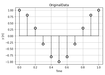
元の離散データはこのような1秒間に１周するデータです。

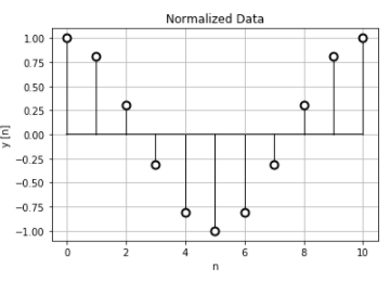
このデータを正規化すると、横軸が時間ではなく、データカウント\(n=0,1,2,3, \cdots\)になります。このデータで離散時間フーリエ変換を計算します。

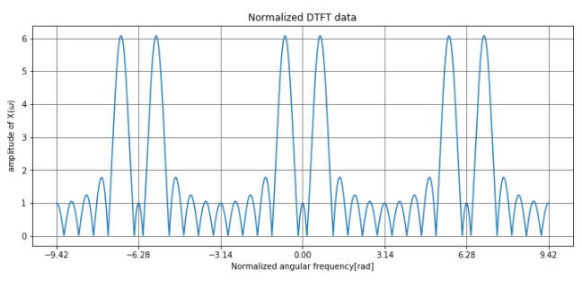
周期性を確認するために3周期分計算したデータです。ちゃんと(2 \pi\)で周期的なデータになっています。このグラフは横軸が正規化されているので、何Hzにインパルスがあるのかよくわかりません。

そこで、横軸を非正規化周波数\([Hz]\)に変え、複素数であるDTFTデータの振幅、実数部、虚数部を表すと、実部では1Hzが大きくなっていることが分かります。

この１周期分のDTFTデータを使い、離散時間フーリエ逆変換を計算すると、正規化された離散データとほぼ同じになります。

例2 周波数: 1 Hz + 3 Hz, Sampling Frequency: 25 Hz

1Hzと3Hzの\(cos\)信号を足し合わせたデータの離散時間フーリエ変換を計算します。

DataFreq1 = 1 # Hz
DataFreq2 = 3 # Hz
samplingFreq = 25 # Hz
phaseOffset = 0 # rad


time = np.arange(0,1+1/samplingFreq,1/samplingFreq)
y1 = np.cos(2*np.pi*DataFreq1*time + phaseOffset)
y2 = np.cos(2*np.pi*DataFreq2*time + phaseOffset)

y = y1+y2

coswave_DTFT = DTFTManager(time, y, xtick=1)
coswave_DTFT.auto()

元の離散データは1Hzと3Hzの信号が足されたものです。

この正規化時間データで離散時間フーリエ変換を計算します。

例1よりもサンプリング周波数が高いので、振幅データもより多くの櫛状形が現れています。

非正規化周波数[Hz]に変換したデータで確認すると、実部が1Hzと3Hzでピークとなっていることが分かります。振幅もその付近にピークがあります。

離散時間フーリエ逆変換を行うと、正規化時間での離散データが計算できました。

\(sin\)関数の離散時間フーリエ変換

\(sin\)関数を離散時間フーリエ変換を行うと、\(cos\)関数と同じく、その周期\(a\)にインパルスが現れるような結果になります。そして、その結果は虚数部に現れるます。

$$
DTDF[sin(an)] = \frac{\pi}{i} \left[ \sigma(\omega – a) – \sigma(\omega +a) \right]
$$

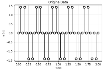
例1 周波数: 2.5Hz , Sampling Frequency: 8 Hz

DataFreq = 2.5 # Hz
samplingFreq = 8 # Hz
phaseOffset = 0 # rad


time = np.arange(0,1+1/samplingFreq,1/samplingFreq)
y = np.sin(2*np.pi*DataFreq*time + phaseOffset)

sinwave_DTFT = DTFTManager(time, y, xtick=0.5)
sinwave_DTFT.auto()

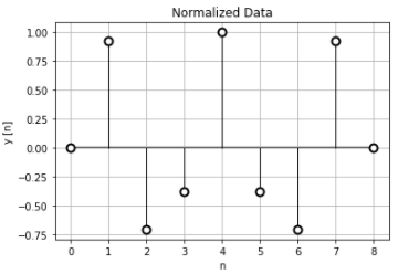
元の離散データは周期とサンプリング周波数が整合を取れないような関係なので、人間の目では\(sin\)関数にはなかなか見えません。

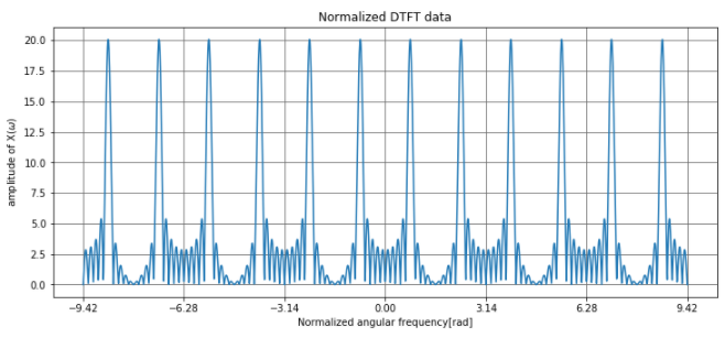
次の正規化時間データで離散時間フーリエ変換を計算します。

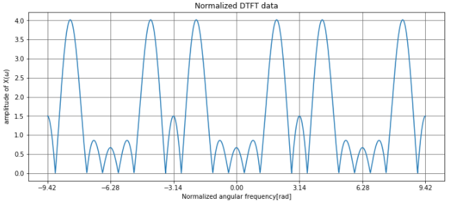
当たり前ですが、離散時間フーリエ変換の値は\(2\pi\)周期で繰り返されています。

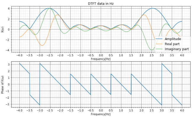
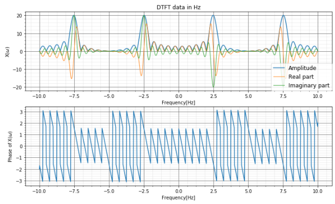
非正規化周波数[Hz]のデータで見てみると、虚数部が2.5Hzでピークとなっていることが分かりますね。振幅もこの2.5Hz付近でピークとなっています。もとの離散データが人間の目で分かりにくくても、計算させればこのように解析することが出来ます。

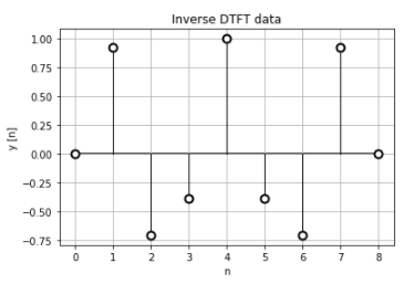
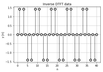
離散時間フーリエ逆変換を行っても、元の正規化時間離散データとほぼ同じになっています。

例2 周波数: 2.5Hz + 7.5 Hz , Sampling Frequency: 20 Hz

2.5 Hzと 7.5Hzの\(sin\)関数を足し合わせた離散データを離散時間フーリエ変換をおこなってみます。

DataFreq1 = 2.5 # Hz
DataFreq2 = 7.5 # Hz
samplingFreq = 20 # Hz
phaseOffset = 0 # rad


time = np.arange(0,1+1/samplingFreq,1/samplingFreq)
y1 = np.sin(2*np.pi*DataFreq1*time + phaseOffset)
y2 = np.sin(2*np.pi*DataFreq2*time + phaseOffset)

y = y1 + y2

sinwave_DTFT = DTFTManager(time, y, xtick=2.5)
sinwave_DTFT.auto()

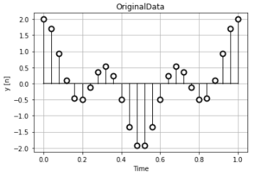
元の離散データです。例1と同じく、やはり人の目にはピンとこないデータです。

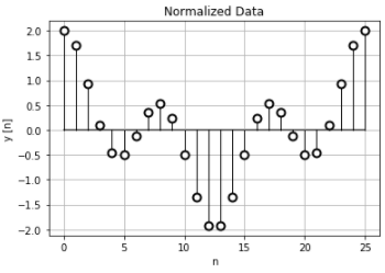
そしてこの正規化時間のデータで離散時間フーリエ変換を行います。

離散時間フーリエ変換のデータは\(2 \pi\)周期で繰り替えされています。

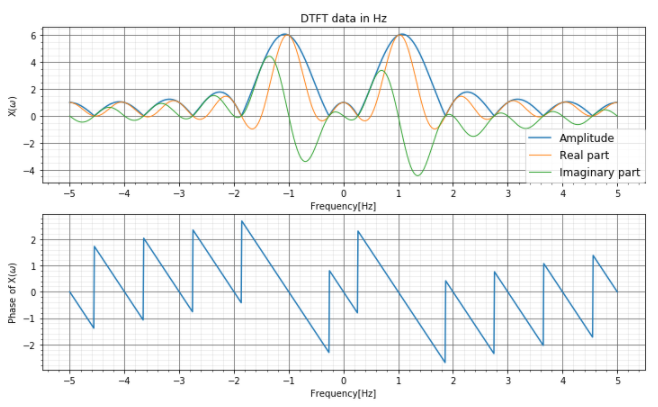
非正規化周波数[Hz]で確認すると、2.5Hzと7.5Hzでピークになっていますね。\(sin\)関数の離散時間フーリエ変換は虚数部の負がその結果になるので、以下のグラフでも虚数部のマイナス側が離散時間フーリエ変換の結果がプラス側になっています。

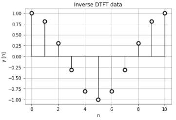
離散時間フーリエ逆変換の結果も、元の離散データの正規化時間データとほぼ一致しています。

インパルス関数 \(\sigma\)の離散時間フーリエ変換

\(\sigma[n-M]\)の離散時間フーリエ変換を計算します。

\(M=0\)の場合

\(M=0\)の場合、\(\sigma[n]\)の離散時間フーリエは”1″になります。

$$
DTFT[\sigma[n-M]] = DTFT[\sigma[n]] = 1
$$

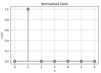
xd_n = np.array([1,0,0,0,0,0,0])
n_array =  np.arange(start = 0, stop = len(xd_ori))


impluse_man = DTFTManager(n_array, xd_n)
impluse_man.auto()

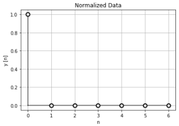
離散データは既に正規化時間データになっていると考えます。

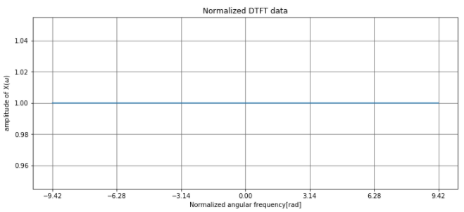
離散時間フーリエ変換の結果は、すべての周波数で”1″となっています。

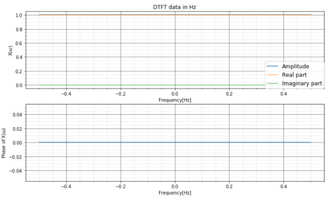
非正規化周波数のデータで確認すると、実部が常に1で、虚数部が常にゼロです。また、位相も常に０です。これは、振幅と位相が周波数に依存しない値となっていることを示しています。

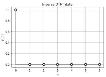
離散時間フーリエ逆変換の結果も、n=0で”1″、それ以外はゼロとなり、元のデータと一定しています。

\(M=1\)の場合

\(M \neq 0\)の場合、離散時間フーリエ変換の結果は、周波数\(\omega\)に依存する関数になります。\(M=1\)ならば、1周期で１周するようなデータになります。

$$
DTDF[\sigma[n-M]] = e^{-i \omega M}
$$

xd_n = np.array([0,1,0,0,0,0,0])
n_array =  np.arange(start = 0, stop = len(xd_ori))


impluse_man = DTFTManager(n_array, xd_n)
impluse_man.auto()

正規化時間データは、n=1が”1″となるデータです。

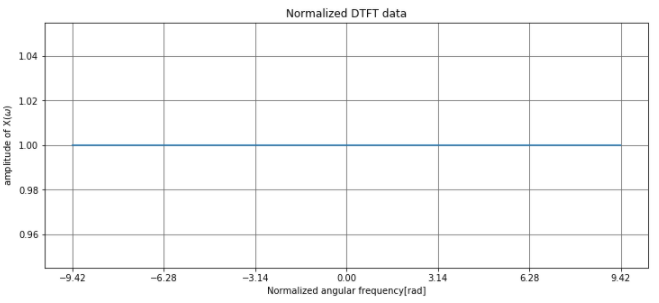
このデータの離散時間フーリエ変換の結果は、振幅は変化していないので、常に1になります。

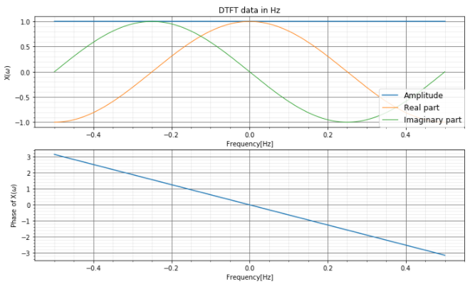
正規化周波数[Hz]で確認すると、実部が\(cos\)、虚数部が\(sin\)となっているので、\(e^{-i \omega} = \cos(\omega) – i \sin(\omega) \)の関係になっていることが分かります。

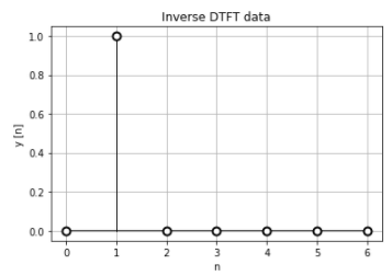
離散時間フーリエ逆変換の結果は、正規化時間データと同じになります。

\(M=2\)の場合

\(M \neq 0\)の場合、離散時間フーリエ変換の結果は、周波数\(\omega\)に依存する関数になります。\(M=2\)ならば、1周期で2周するようなデータになります。

$$
DTDF[\sigma[n-M]] = e^{-i \omega M}
$$

xd_n = np.array([0,0,1,0,0,0,0])
n_array =  np.arange(start = 0, stop = len(xd_ori))


impluse_man = DTFTManager(n_array, xd_n)
impluse_man.auto()

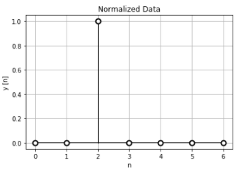
正規化時間データは n=2が”1″になっています。

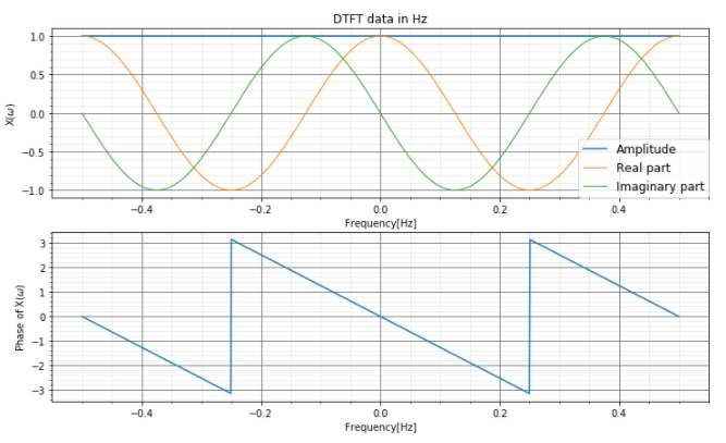
このデータを離散時間フーリエ逆変換し、１周期分の非正規化周波数[Hz]を確認すると、実部と虚部が１周期の間に２周していることが分かります。つまり、\(e^{-i 2 \omega} = cos(2 \omega) -i sin (2 \omega) \)になっています。

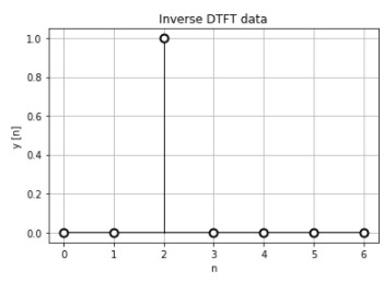
離散時間フーリエ逆変換の結果は正規化時間データと一致する形です。

数列の離散時間フーリエ変換

例1 次の値は前の値の半分になる

次の式のような数列を離散時間フーリエ変換を計算します。

$$
\left\{
\begin{array}{l l}
0 & n = 0 \\
\frac{1}{2^{n-1}} & elsewhere
\end{array}
\right.
$$

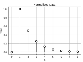
xd_ex1 = np.array([0,1,1/2,1/4,1/8,1/16,1/32,1/64,1/128])
n_ex1 =  np.arange(start = 0, stop = len(xd_ex1))


ex2_DTFT = DTFTManager(n_ex1, xd_ex1)
ex2_DTFT.auto()

離散時間フーリエ変換を行うデータは、以下のようなデータです。さて、どんな結果になるでしょうか？

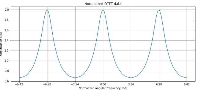
周波数ゼロを中心に振幅が下がるような形をしています。これは、ゼロ付近の低周波側の振幅が大きく、高周波側である\(\pi\)に近づくほど振幅が小さくなっているので、ローパスフィルタのようになっていることが分かりますね。

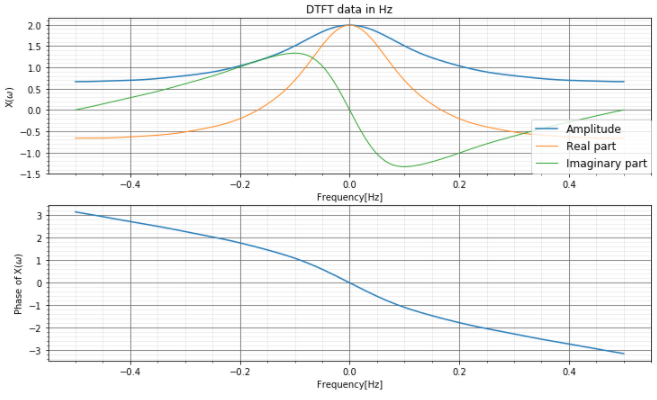
非正規化周波数で１周期分を確認すると、こんな感じになっています。下段の位相データを確認すると、高周波について位相が遅れているのでローパスフィルタと同じ挙動を示しています。

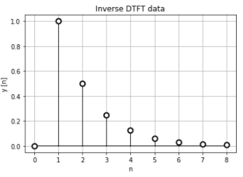
もちろん離散時間フーリエ逆変換の結果は元の数列に戻ります。

例2 正負を繰り返しながら収束する

数式だとこんな感じの式になります。Wikipediaによると、この数列は微分回路フィルタとして機能するようです。

$$
DTFT\left[\left\{
\begin{array}{l l}
0 & n = 0 \\
\frac{(-1)^n}{n} & elsewhere
\end{array}
\right.\right] = j \omega
$$

def createNumArray(n):
    xn = np.zeros(n+1)
    n_array = np.arange(n+1)
    for i in range(n+1):
        if i == 0:
            value = 0
        else:
            value = math.pow(-1,i) / i
        
        xn[i] = value
    
    return n_array , xn


n_array, xn = createNumArray(15)

man = DTFTManager(n_array, xn)
man.auto()

グラフで確認すると、このような離散データです。

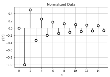
３周期分の離散時間フーリエ変換を確認すると、ゼロ付近が少なく、\(\pi\)近くの高周波側の振幅が大きくなっています。ここから、微分回路フィルタとして機能する、つまり、低周波信号を微分してもほとんど変化が無いので振幅が少なく、高周波信号を微分すると変化が大きいので振幅が多いので、ハイパスフィルタとして働くと考えられます。

非正規化周波数Hzの１周期分で確認すると、上の変換式の関係通り、\(j \omega\)となっていますね。ちょっとガタガタしていますが、虚数部が周波数に応じた変化をしていますね。

離散時間フーリエ逆変換の結果はもちろん正規化時間データと一致しています。

リクエスト受け付けています

色々なデータを離散時間フーリエ変換と離散時間フーリエ逆変換を行ってみました。

ネットで色々探してみましたが、ここまで詳しく計算しているサイトは大学も含めて見つけることが出来ませんでした。

他にももしかして困っている方がいるかなと思うので、コメント欄に”こんな数列を離散時間フーリエ変換して見せてほしい”等を書いてもらえれば計算してみます。

何か質問あれば、お気軽にコメントくださいね